Census Dataset Analysis

The United States Census of 2018 collected broad information about the US Government employees, including demographic information $Z$ ($Z_1$ for age, $Z_2$ for race, $Z_3$ for nationality), gender $X$ ($x_0$ female, $x_1$ male), marital and family status $M$, education information $L$, and work-related information $R$.

A data scientist loads the data and performs the following initial analysis:

data <- get(data("gov_census", package = "faircause"))
data <- as.data.frame(data[seq_len(20000)])
knitr::kable(head(data), caption = "Census dataset.")

Census dataset.
sex	age	race	hispanic_origin	citizenship	nativity	marital	family_size	children	education_level	salary	hours_worked	weeks_worked	occupation	industry	economic_region
male	64	black	no	1	native	married	2	0	20	43000	56	49	13-1081	928P	Southeast
female	54	white	no	1	native	married	3	1	20	45000	42	49	29-2061	6231	Southeast
male	38	black	no	1	native	married	3	1	24	99000	50	49	25-1000	611M1	Southeast
female	41	asian	no	1	native	married	3	1	24	63000	50	49	25-1000	611M1	Southeast
female	40	white	no	1	native	married	4	2	21	45200	40	49	27-1010	611M1	Southeast
female	46	white	no	1	native	divorced	3	1	18	28000	40	49	43-6014	6111	Southeast

mean_sal <- tapply(data$salary, data$sex, mean)
tv <- mean_sal[2] - mean_sal[1]

Therefore, the data scientist observed that male employees on average earn $14000/year more than female employees, that is

$E[y \mid x_1] - E[y \mid x_0] = 15054.$

Following the Fairness Cookbook, the data scientist does the following:

SFM projection: the SFM projection of the causal diagram $\mathcal{G}$ of this dataset is given by \[ \Pi_{\text{SFM}}(\mathcal{G}) = \langle X = \lbrace X \rbrace, Z = \lbrace Z_1, Z_2, Z_3 \rbrace, W = \lbrace M, L, R\rbrace, Y = \lbrace Y \rbrace\rangle. \] She then inputs this SFM projection into the faircause R-package,

set.seed(2022)
mdata <- SFM_proj("census")
mdata

$X
[1] "sex"

$W
[1] "marital"         "family_size"     "children"        "education_level"
[5] "english_level"   "hours_worked"    "weeks_worked"    "occupation"     
[9] "industry"       

$Z
[1] "age"             "race"            "hispanic_origin" "citizenship"    
[5] "nativity"        "economic_region"

$Y
[1] "salary"

$x0
[1] "male"

$x1
[1] "female"

$ylvl
[1] NA

fc_census <- fairness_cookbook(
  as.data.frame(data), X = mdata$X, Z = mdata$Z, W = mdata$W,
  Y = mdata$Y, x0 = mdata$x0, x1 = mdata$x1
)

autoplot(fc_census, decompose = "xspec", dataset = "Census")

Figure 1: Fairness Cookbook on the Census dataset.

Using these results, she considers the following:

Disparate treatment: when considering disparate treatment, she computes $x\text{-DE}_{x_0, x_1}(y \mid x_0)$ and its 95% confidence interval to be

$x\text{-DE}_{x_0, x_1}(y \mid x_0) = -10891\pm443.$

The hypothesis $H_0^{(x\text{-DE})}$ is thus rejected, providing evidence of disparate treatment of females.

Disparate impact: when considering disparate impact, she notice that Ctf-SE, Ctf-IE and their respective 95% confidence intervals equal:

$\begin{align}x\text{-IE}_{x_1, x_0}(y \mid x_0) &= 5190\pm342\\x\text{-SE}_{x_1, x_0}(y) &= -1027\pm435.\end{align}$

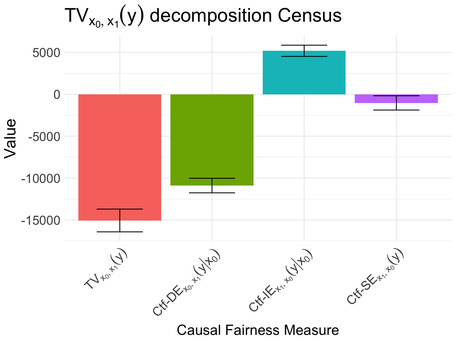
The data scientist decides that the differences in salary explained by the spurious correlation of gender with age, race, and nationality are not considered discriminatory. Therefore, she tests the hypothesis \[H_0^{(x\text{-IE})}: x\text{-IE}_{x_1, x_0}(y \mid x_0) = 0,\] which is rejected, indicating evidence of disparate impact on female employees of the government. The measures computed in this example are visualized in Figure 1.