col_adm <- function(n, cfs, kap = cfs[["kap"]], lam = cfs[["lam"]],
                    alf = cfs[["alf"]], bet = cfs[["bet"]]) {

  u_xz <- rbinom(n, size = 1, prob = 0.5)
  x <- rbinom(n, size = 1, prob = 0.5 + 0.1 * u_xz)
  z <- rbinom(n, size = 1, prob = 0.5 + kap * u_xz)
  d <- rbinom(n, size = 1, prob = 0.5 + lam * x)
  y <- rbinom(n, size = 1, prob = 0.1 + alf * x + bet * d + 0.1 * z)

  data.frame(x, z, d, y)

}

cfs_nxt <- function(cfs, kap = cfs[["kap"]], lam = cfs[["lam"]],
                    alf = cfs[["alf"]], bet = cfs[["bet"]]) {

  kapt <- kap * 0.9
  lamt <- lam * (1 - bet)
  bett <- bet * (1 - lam) * runif(1, 0.8, 1.2)
  alft <- alf * 0.8

  list(kap = kapt, lam = lamt, alf = alft, bet = bett)

}College Admissions: Task 1 over Time
College Admissions: Bias Detection over Time
In this vignette, we analyze a synthetic College Admission dataset, to demonstrate how the task of bias detection could be performed over time, in a university. In particular, we have the following story.
A university in the United States admits applicants every year. The university is interested in quantifying discrimination in the admission process and track it over time, between 2010 and 2020. The data generating process changes over time, and can be described as follows. Let \(X\) denote gender (\(x_0\) female, \(x_1\) male). Let \(Z\) be the age at time of application (\(Z = 0\) under 20 years, \(Z = 1\) over 20 years) and let \(W\) denote the department of application (\(W = 0\) for arts&humanities, \(W = 1\) for sciences). Finally, let \(Y\) denote the admission decision (\(Y = 0\) rejection, \(Y = 1\) acceptance). The application process changes over time and is given by \[ \begin{empheq}[left ={\mathcal{F}(t), P(U): \empheqlbrace}]{align} X & \gets \mathbb{1} ( U_X < 0.5 + 0.1U_{XZ})\label{eq:fcb2-x}\\ Z & \gets \mathbb{1} (U_Z < 0.5 + \kappa(t) U_{XZ}) \\ W & \gets \mathbb{1} (U_W < 0.5 + \lambda(t) U_{XZ}) \\ Y & \gets \mathbb{1} (U_Y < 0.1 + \alpha(t)X + \beta(t)W + 0.1Z). \label{eq:fcb2-y} \\ \nonumber\\ U_{XZ} &\in \{0,1\}, P(U_{XZ} = 1) = 0.5, \\ U_X &, U_Z, U_W, U_Y \sim \text{Unif}[0, 1]. \end{empheq} \] The coefficients \(\kappa(t), \lambda(t), \alpha(t), \beta(t)\) change every year, and obey the following dynamics: \[ \begin{align} \kappa(t+1) &= 0.9\kappa(t) \\ \lambda(t+1) &= \lambda(t) (1 - \beta(t)) \\ \beta(t+1) &= \beta(t) (1 - \lambda(t)) f(t), f(t) \sim \text{Unif}[0.8, 1.2] \\ \alpha(t+1) &= 0.8\alpha(t). \end{align} \] The equations can be interpreted as follows. The coefficient \(\kappa(t)\) decreases over time, meaning that the overall age gap between the groups decreases. The coefficient \(\lambda(t)\) decreases compared to the previous year, by an amount dependent on \(\beta(t)\). In words, the rate of application to arts&humanities departments decreases if these departments have lower overall admission rates (i.e., students are less likely to apply to departments that are hard to get into). Further, \(\alpha(t)\), which represents gender bias, decreases over time. Finally, \(\beta(t)\) represent the increase in the probability of admission when applying to a science department. Its value depends on the value from the previous year, multiplied by \((1 - \lambda(t))\) and the random variable \(f(t)\). Multiplication by the former factor describes the mechanism in which the benefit of applying to a science department decreases if a larger proportion of students apply for it. The latter factor describes a random variation over time which describes how well (in relative terms) the science departments are funded, and can be seen as depending on research and market dynamics in the sciences.
We now create functions for generating synethetic data as described above:
The head data scientist at the university decides to use the Fairness Cookbook for performing bias quantification. The SFM projection of the causal diagram \(\mathcal{G}\) of the dataset is given by \[ \begin{equation} \Pi_{\text{SFM}}(\mathcal{G}) = \langle X = \lbrace X \rbrace, Z = \lbrace Z \rbrace, W = \lbrace W\rbrace, Y = \lbrace Y \rbrace\rangle. \end{equation} \] After that, the analyst estimates the quantities \[ \begin{align} x\text{-DE}^{\text{sym}}_{x}(y \mid x_0), x\text{-DE}^{\text{sym}}_{x}(y \mid x_0), \text{ and } x\text{-SE}_{x_1, x_0}(y) \;\;\; \forall t \in \{2010, \dots, 2020\}. \end{align} \]
The following code generates the data, obtains the ground truth causal fairness measures, and also performs the fairness_cookbook() at each step.
col_adm_tim <- function(n, cfs) {

  dat <- bqn <- gtr <- list()

  for (t in seq_len(10)) {

    # generate data for given year
    dat[[t]] <- col_adm(n, cfs)

    # compute decomposition
    bqn[[t]] <- fairness_cookbook(dat[[t]], X = "x", Z = "z", W = "d", Y = "y",
                                  x0 = 0, x1 = 1)

    # get ground truth
    gtr[[t]] <- c(cfs$alf, -(cfs$bet * cfs$lam),
                  0.1 * ( (0.125 + 0.2 * (0.5 + cfs$kap))/(0.45) -
                             (0.125 + 0.4 * (0.5 + cfs$kap))/(0.55) ))

    # update the coefficients for each year
    cfs <- cfs_nxt(cfs)

  }

  list(dat = dat, bqn = bqn, gtr = gtr)

}

cfs <- list(kap = 0.3, lam = 0.2, alf = 0.1, bet = 0.3)

set.seed(22)
res <- col_adm_tim(n = 5000L, cfs = cfs)

otp <- c()
for (t in seq_along(res[["bqn"]])) {

  x <- summary(res[["bqn"]][[t]])$measures
  x_tr <- res[["gtr"]][[t]]
  add_row <- data.frame(
    Spurious = x[x$measure == "ctfse", ]$value,
    Indirect = x[x$measure == "ctfie", ]$value,
    Direct = x[x$measure == "ctfde", ]$value,
    Spurious_True = x_tr[3],
    Indirect_True = x_tr[2],
    Direct_True = x_tr[1],
    Year = 2010+t
  )

  otp <- rbind(otp, add_row)

}

df <- reshape2::melt(otp, id.vars = "Year", variable.name = "Measure")
df$Meas <- gsub("_.*", "", df$Measure)
df$whc <- ifelse(grepl("_", df$Measure), "True (population)",
                 "Estimated (from sample)")

ggplot(df, aes(x = Year, y = value, color = Meas, linetype = whc)) +
  geom_line() + geom_point() + theme_bw() +
  ggtitle("Bias Quantification Over Time - College Admissions") +
  ylab("Value") + scale_y_continuous(labels = scales::percent,
                                     limits = c(-0.1, 0.15)) +
  scale_x_continuous(breaks = seq(2010, 2020)) +
  theme(
    legend.position = "bottom",
    legend.box.background = element_rect(),
    legend.box = "horizontal"
  ) + scale_linetype_discrete(name = "Quantity") +
  scale_color_discrete(name = "Effect")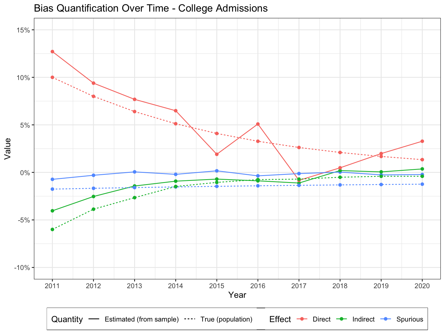
The temporal dynamics of the estimated measures of discrimination (together with the ground truth values obtained from the SCM \(\mathcal{M}_t\)) are shown graphically in Figure 1.