Fair Predictions can be obtained by passing the data, SFM, and the choice of the business necessity set (BN) to the fair_predictions() function:
# build our own predictor and decompose the true onefair_pred <-fair_predictions(data, X, Z, W, Y, x0 =0, x1 =1,BN =c("IE"))
Note that in faircause 0.2.0 the columns of the input data to functions fair_predictions() and fair_decisions() need to be either numeric or integer. Use one-hot encoding wherever appropriate.
When fitting the fair predictor, pytorch is used under the hood to optimize the function of the form: \[
\begin{align}
L(y, \hat{y}) + \lambda \Big( | \text{NDE}_{x_0, x_1}(\hat{y}) - \eta_1 | + | \text{NIE}_{x_1, x_0}(\hat{y}) - \eta_2 | + | \text{Exp-SE}_{x_1}(\hat{y}) - \eta_3 | + | \text{Exp-SE}_{x_0}(\hat{y}) - \eta_4 | \Big)
\end{align}
\] where the values \(\eta_1, \eta_2, \eta_3, \eta_4\) are either 0 if effect is not in the business necessity set, or equal the effect estimate for the true outcome \(Y\) (if the effect is BN). Multiple values of the tuning parameter \(\lambda\) are used at the same time (this choice can also be adjusted using the lmbd_seq parameter, to which an arbitrary sequence of values can be passed). For binary classification the loss \(L(y, \hat{y})\) is the cross-entropy, whereas for regression the loss is the mean squared error (MSE).
In the above, fair_pred is S3-class object of type fair_prediction. We can use the predict() function to obtain its predictions on new data.
preds <-predict(fair_pred, data)# appending the in-sample predictions to the datasetdata$faircause_preds <- preds$predictions[[5]]
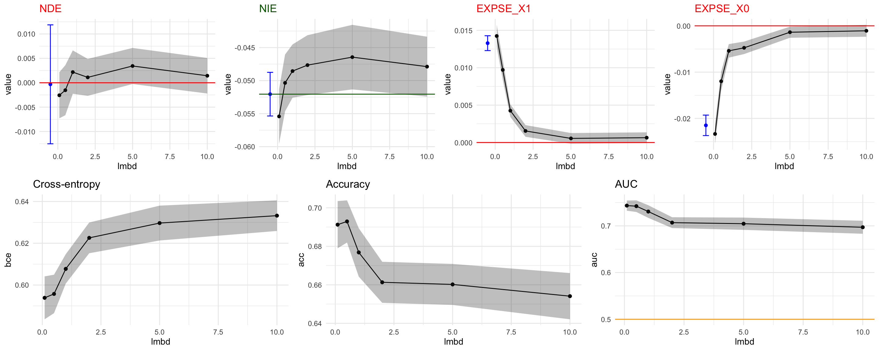
Further generics can be applied to fair_prediction objects, such as autoplot(), which allows us to visualize the loss function and the causal fairness measures on held-out evaluation data:
cowplot::plot_grid(autoplot(fair_pred, type ="causal"),autoplot(fair_pred, type ="accuracy"), ncol = 1L)
Decomposing the Disparity on Evaluation Data
The function fair_prediction() takes an eval_prop argument which determines the proportion of data that is used as an evaluation fold (for early stopping when fitting the neural network). We now extract this fold of the data, and decompose the disparity manually:
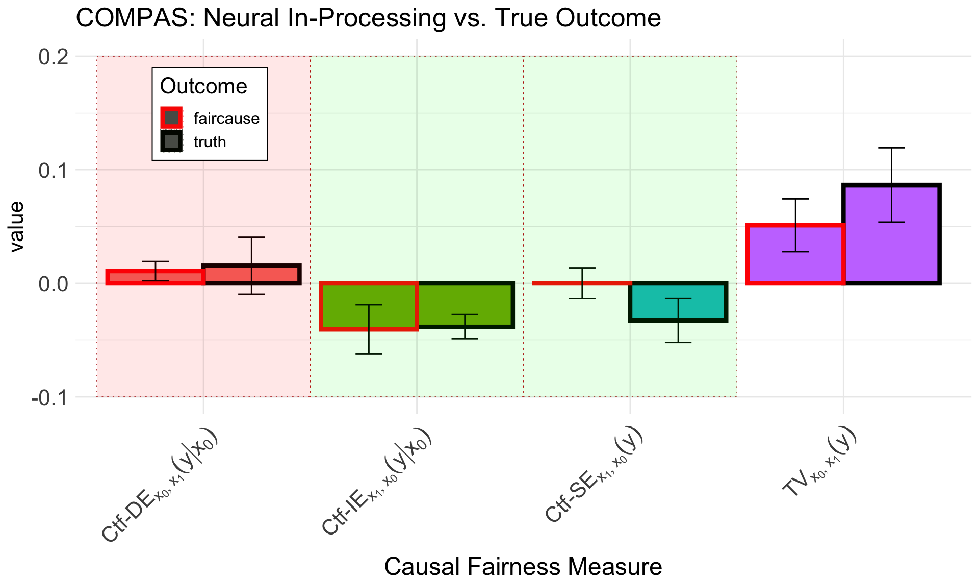
# decompose the predictions on the eval settrain_idx <-seq_len(round(0.75*nrow(data)))faircause_decomp <-fairness_cookbook(data[-train_idx,], X = X, W = W, Z = Z,Y ="faircause_preds",x0 =0, x1 =1, nboot1 =20, nboot2=100)
Finally, we can plot the two decompositions, of the true outcome \(Y\) and the newly constructed causally fair predictor \(\widehat{Y}^{FC}\), together: