COMPAS - Task 1
In this vignette, we generalize the analysis of the Fairness Cookbook, to consider more refined settings described by an arbitrary causal diagram. The main motivation for doing so comes from the observation that when analyzing disparate impact, quantities such as Ctf-DE\(_{x_0,x_1}(y\mid x_0)\), Ctf-IE\(_{x_0,x_1}(y\mid x_0)\), and Ctf-SE\(_{x_0,x_1}(y)\) are insufficient to account for certain business necessity requirements. For concreteness, consider the following example.
COMPAS under Business Necessity
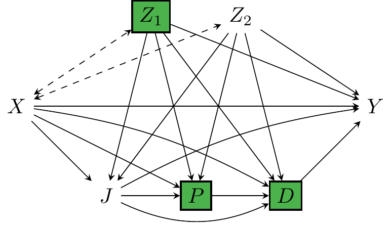
The courts at Broward County, Florida, were using machine learning to predict whether individuals released on parole are at high risk of re-offending within 2 years. The algorithm is based on the demographic information \(Z\) (\(Z_1\) for gender, \(Z_2\) for age), race \(X\) (\(x_0\) denoting White, \(x_1\) Non-White), juvenile offense counts \(J\), prior offense count \(P\), and degree of charge \(D\).
A causal analysis using the fairness_cookbook() revealed that:
data <- get(data("compas", package = "faircause"))
set.seed(2022)
mdata <- SFM_proj("compas")
fc_compas <- fairness_cookbook(data, X = mdata$X, Z = mdata$Z, W = mdata$W,
                               Y = mdata$Y, x0 = mdata$x0, x1 = mdata$x1)

autoplot(fc_compas, decompose = "xspec", dataset = "COMPAS")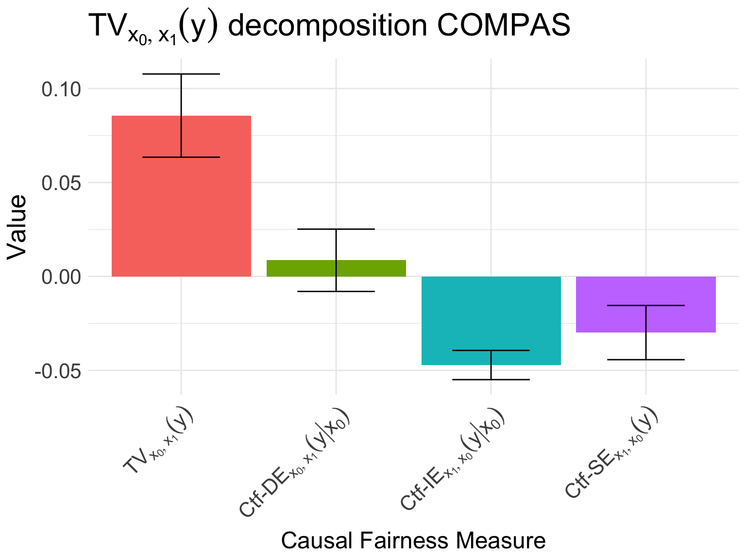
That is, the computed measures equal: \[ \begin{align} \text{Ctf-IE}_{x_1, x_0}(y\mid x_1) &= -5.7\% \pm 0.5\%,\\ \text{Ctf-SE}_{x_1, x_0}(y) &= -4.0\% \pm 0.9\%, \end{align} \] and are also shown graphically in Figure 2, potentially indicating presence of disparate impact. Based on this information, a legal team of ProPublica filed a lawsuit to the district court, claiming discrimination w.r.t. the Non-White subpopulation based on the doctrine of disparate impact. After the court hearing, the judge rules that using the attributes age (\(Z_2\)), prior count (\(P\)), and charge degree (\(D\)) is not discriminatory, but using the attributes juvenile count (\(J\)) and gender (\(Z_1\)) is discriminatory. The causal diagram with a visualization of which variables are included in the business-necessity set is given in Figure 1. Data scientists at ProPublica need to consider how to proceed in the light of this new requirement for discounting the allowable attributes in the quantiative analysis.
The difficulty in this example is that the quantity Ctf-SE\(_{x_1, x_0}(y)\) measures the spurious discrimination between the attribute \(X\) and outcome \(Y\) as generated by both confounders \(Z_1\) and \(Z_2\). Since using the confounder \(Z_2\) is not considered discriminatory, but using the confounder \(Z_1\) is, the quantity Ctf-SE\(_{x_1, x_0}(y)\) needs to be refined such that the spurious variations based on the different confounders are disentangled. In particular, one might be interested in finding a decomposition of the spurious effect such that \[ \begin{align} \text{Ctf-SE}_{x_1, x_0}(y) = \underbrace{\text{Ctf-SE}^{Z_1}_{x_1, x_0}(y)}_{\text{gender variations}} + \underbrace{\text{Ctf-SE}^{Z_2}_{x_1, x_0}(y)}_{\text{age variations}}, \end{align} \] which would allow the data analyst to further distinguish the variations explained by each of the confounders. A similar challenge is present for the Ctf-IE\(_{x_1, x_0}(y\mid x_1)\) measure, since it has contributions explained by juvenile offense counts \(J\), prior counts \(P\), and the charge degree \(D\). Therefore, we might be interested in decomposing the indirect effect into \[ \begin{align} \text{Ctf-IE}_{x_1, x_0}(y \mid x_1) =& \underbrace{\text{Ctf-IE}^J_{x_1, x_0}(y \mid x_1)}_{\text{juvenile count variations}} + \underbrace{\text{Ctf-IE}^P_{x_1, x_0}(y \mid x_1)}_{\text{prior count variations}} \\ &+ \underbrace{\text{Ctf-IE}^D_{x_1, x_0}(y \mid x_1)}_{\text{charge degree variations}}. \nonumber \end{align} \] Again, such a decomposition would allow the data analyst to better understand the contribution of each of the mediators to the totality of the indirect effect. In situations when some mediating variables are in the business necessity set, while others are not, such a decomposition would allow for assessment of disparate impact claims.